Active seismic regions release their tectonic strain mostly through earthquakes of different magnitudes on faults and subduction zones. For hazard analysis, it is necessary to quantify the rates of occurrences of these different magnitude earthquakes on different regional seismic sources. Seismologists refer to this process as building magnitude-rate distributions (MRDs) for seismic sources. The most common MRD used in practice is the Gutenberg-Richter (GR) distribution which was developed by Charles Francis Richter and Beno Gutenberg in 1944 based on California earthquake data.
It is the fact of nature that large magnitude earthquakes occur less frequently than the small ones. In other words, the rates of occurrences of earthquakes decrease with increasing magnitude.
$$n=-\frac{dN}{dM}… (1)$$
where \( \frac{dN}{dM} \) is the change in the rate of occurrence per unit magnitude identified by \(n\), known as the density function. Note that \(N\) for any given magnitude \(M_0\) defines the occurrence rate of earthquakes of magnitudes \(M \ge M_0\). The negative sign signifies the fact the rates of earthquakes decrease with the increasing magnitude.
The GR distribution defines the density function as
$$n=10^{a-b * M}…(2)$$
where \(a\) and \(b\) are region dependent constants that control the level of seismicity and the change in the rate of occurrence with magnitude, respectively. Using equations 1 and 2, the total number of earthquakes within the magntide range of \(dM\) can be estimated as
$$dN= 10^{a-b * M}*dM…(3)$$
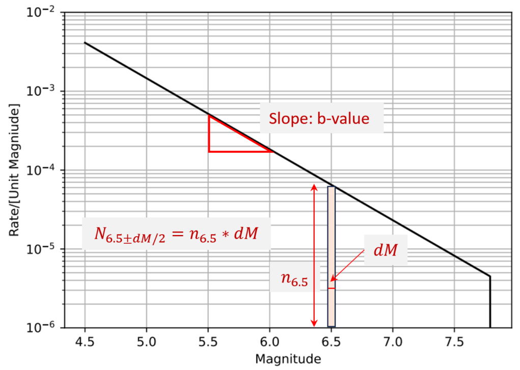
Figure 1 shows a plot of \(log(n)=a-b*M\) as a function of magnitude. The \(b-value\) defines the slope of the curve which characterizes the relative rates of occurrences of large and small magnitude earthquakes. Sources with low \(b-value\) release more of their strain energy by large magnitude earthquakes compared to the sources with high \(b-value\). The typical \(b-value\) for most regions is within \(0.8 – 1.2\).
The \(a-value\) defines the scale of seismicity and can be estimated by the value of \(n\) at \(M = 0\) in equation 3. For example, in the last two US national seismic hazard models USGS reported background seismicity at grids as the rate of earthquakes of magnitude \(-0.05 \le M \le 0.05\) (\(M = 0 \pm 0.05\)). Accordingly, the \(a-value\) can be estimated as \(a=log(N_{0 \pm 0.05} /0.1)\). Using the estimated \(a-value\) in conjunction with the \(b-value\) and the upper bound magnitude, both provided by the USGS, one can fully construct the GR magnitude-rate density distributions for all grids.
The occurrence rate of earthquakes of magnitudes \(\ge M\) can be estimated as
$$N=-\int_{M}^{M_{max}} {n*dM}…(4)$$
Using the formulation of the density function from equation 2, the cumulative rate can be formulated as
$$N=N_0*\frac{{10^{-b*(M-M_0)}-10^{-b*(M_{max}-M_0)}}}{{1-10^{-b*(M_{max}-M_0} )}}…(5)$$
where \(N_0\) is the rate of earthquakes of magnitude \(M \ge M_0\) and \(M_{max}\) is the maximum magnitude considered for the GR distribution.
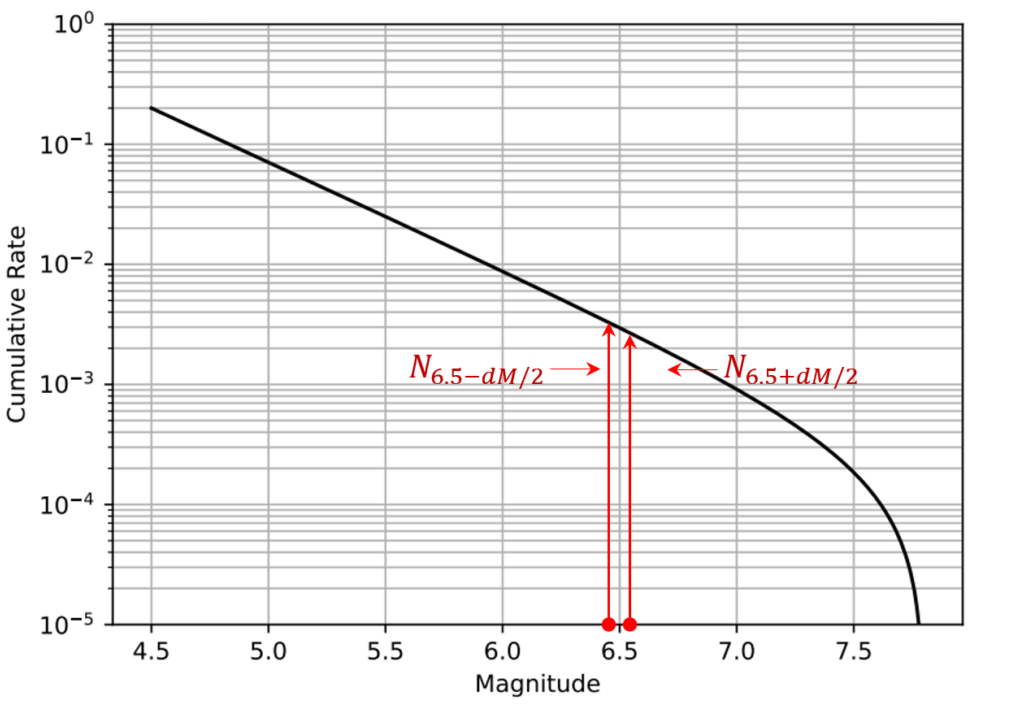
Figure 2. shows the plot of the cumulative magnitude-rate distribution corresponding to the density function in Figure 1. Also shown in these figures are the visual correspondence between the occurrence rate for \(M=6.5 \pm dM/2\) earthquakes using density and cumulative distributions.
Equation 5 and the plot in Figure 2 are known as the truncated MRD. It is called truncated since the MRD is normalized in such a way that as the magnitudes of earthquakes increases the rates of occurrences decreasing and goes to zero at the maximum magnitude.