Sand Box: Construct and evaluate magnitude-rate distribution scenarios
Active seismic regions release accumulated tectonic strain primarily through earthquakes of various magnitudes occurring on faults and subduction zones. For seismic hazard analysis, it is essential to quantify how often earthquakes of different magnitudes occur on each seismic source. Seismologists refer to this process as constructing magnitude–rate distributions (MRDs).
The most widely used MRD in practice is the Gutenberg–Richter (GR) distribution, developed by Charles F. Richter and Beno Gutenberg (1944) based on earthquake observations in California.
1. Fundamental Behavior of Earthquake Occurrence
A basic property of seismicity is that large earthquakes occur less frequently than small ones. This means that the rate of earthquake occurrence decreases as magnitude increases. Mathematically:
$$
n = -\frac{dN}{dM}
$$
where:
- \( dN/dM \) is the change in occurrence rate per unit magnitude,
- \( n \) is the magnitude–rate density function,
- \( N \) is the rate of earthquakes with magnitudes \( M \ge M_{\text{ref}} \).
The negative sign indicates that earthquake rates decline with increasing magnitude.

Figure 1.
2. The Gutenberg–Richter Density Function
The GR distribution defines the density function as:
$$
n = 10^{a – bM}
$$
where:
- \( a \) controls the overall level of seismicity,
- \( b \) controls how rapidly earthquake rates decrease with magnitude.
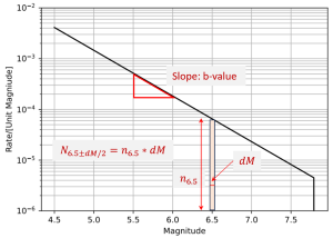
Combining the definition of \( n \) with the GR form gives the expected number of earthquakes in a small magnitude interval \( dM \):
$$
dN = 10^{a – bM}* dM
$$
3. Interpretation of the GR Parameters
The b‑value
Plotting \( log(n) = a – bM \) produces a straight line with slope \( -b \).
The b‑value describes the relative occurrence of small versus large earthquakes:
- Low \( b \) → proportionally more large earthquakes
- High \( b \) → proportionally more small earthquakes
Most regions exhibit \( b \) values between 0.8 and 1.2.
The a‑value
The a‑value sets the absolute scale of seismicity.
At \( M = 0 \):
$$
n(M=0) = 10^{a}
$$
The USGS hazard model reports background seismicity as the rate of earthquakes within:
$$
-0.05 \le M \le 0.05
$$
Using the GR density, the corresponding a‑value is:
$$
a = \log\left(\frac{N_{0\pm0.05}}{0.1}\right)
$$
Once the a‑value, b‑value, and upper‑bound magnitude are known, the full GR magnitude–rate density distribution can be constructed for each grid point.
4. Cumulative Occurrence Rates
The rate of earthquakes with magnitudes \( M \ge M_{\min} \) is obtained by integrating the density function:
$$
N = -\int_{M}^{M_{\max}} n\, dM
$$
Substituting the GR density yields the truncated cumulative GR distribution:
$$
N =N_0{
\frac{10^{-b(M – M_0)} – 10^{-b(M_{\max} – M_0)}}{1 – 10^{-b(M_{\max} – M_0)}}}
$$
where:
- \( N_0 \) is the rate of earthquakes with \( M \ge M_0 \),
- \( M_{\max} \) is the maximum magnitude allowed in the model.

Figure 2.
5. Why the Distribution Is “Truncated”
The cumulative GR distribution is called truncated because:
- the occurrence rate decreases smoothly with increasing magnitude, and
- the rate approaches zero at the maximum magnitude \( M_{\max} \).
This ensures that the model reflects the physical limit on the largest possible earthquake for a given seismic source.